Walking the tightrope: Klein, Patinkin and Schelling on price flexibility and stability

This work entitled “Walking the Tightrope” by Stevan Dohanos was featured on the cover of the Saturday Evening Post, June 11, 1949.

As Paul Samuelson’s first PhD student, Lawrence Klein was well positioned to endorse the view that any macroeconomic models should bridge static and dynamic analyses (see the post on Samuelson’s 1941 article here). In his 1947 Journal of Political Economy article about theories of effective demand (Klein, 1947), he put forward the idea that Keynesian views could only make sense in a dynamic framework in which the fundamental issue was the stability – if it existed – of full employment equilibrium. At the same time, Don Patinkin (Patinkin, 1995: 385), who worked alongside Klein at the Cowles Commission, reinforced the argument in an article published in the American Economic Review (Patinkin, 1948). In this respect, he chose to refer to the so-called “cobweb theorem” (Patinkin, 1948: 560).

Consider a demand curve and a supply curve for a market. When both curves intersect once, the issue is that of stability: whether the market will reach the stationary position or not. That is, whether it will settle down to a unique price that will continue indefinitely to clear it. A simple cobweb diagram allowed Patinkin to underline this issue in a simplified framework which was used to ensure that his message was understood.

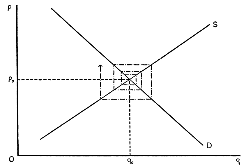
Figure drawn from Patinkin’s 1948 article “price flexibility and full employment” (p.560)

As Patinkin argued, “the question is clearly divided into two parts: a) does there exist such a price, and b) if it does exist, will the market be able to attain it.” (Patinkin 1948: 560). In the case illustrated in the figure above, as long as the price $p_0$ and quantity $q_0$ are maintained, the market remains balanced while if the economy is off that point, the adjustment process is divergent and the equilibrium is never restored.

How could this analysis be applied to the labor market? Both Klein and Patinkin agreed that the introduction of an equation describing the adjustment of money wages was critical to explore the behavior of the economic system. For that purpose, Patinkin (1948, f.n. 33: 562) referred to the following equation, which was at the heart of the discussions that ensued:

$\begin{equation*} \frac{dw}{dt}=f(n^d-n^s) \end{equation*}$

where $\frac{dw}{dt}=\dot w$ is the rate of change of money wages, $n^d$ is the demand for labor and $n^s$ is the supply of labor, so that wage changes depend on unemployment, the difference between the supply and demand of labor (in this equation, since Patinkin used $n^d-n^s$ , the relationship between both sides of the equation is positive). Patinkin and Klein emphasized that nominal wages were the object of effective bargaining, which is why they did not focus on the equation for real wages. Strikingly, neither of them investigated the stability condition of a small-scale macroeconomic model based on such an equation.

Eager to fill that gap, Thomas Schelling came up with his own model and analysis of stability. As he put it in the opening paragraph of his 1950 American Economic Review article:

The purely theoretical case against price flexibility, as a device for restoring or ensuring full employment, has recently come to hinge on dynamic considerations, specifically on the speculative reaction to price changes. Mr. Don Patinkin and Mr. Lawrence Klein have both stated this position. They argue that, while there may at moment be a price level which, if sustained, would yield full employment, the movement of prices toward that level would set off adverse reactions which would dominate the system, causing an aggravation rather than amelioration of unemployment (Schelling, 1949: 911).

Schelling’s argument in his paper was that the instability caused by wage cuts was only temporary, and that the system would return to its equilibrium. In his reply to Schelling, Klein attempted to clear up his argument to show why wage cuts led to instability, although the model he built still remained limited to the labor market. Klein considered the relationship between wage changes and unemployment, to determine how unemployment was influenced by wage expectations and the wage level, which were clearly separated in his analysis.

(1) $\begin{equation*} \frac{dw}{dt}=\alpha_0+\alpha_1 u_t \end{equation*}$

where $u_t$ is unemployment, that is, the difference between the current demand for labor and the current supply of labor.

The demand for labor equation is:

(2) $\begin{equation*} n^d_t = \gamma_0 + \gamma_1 (w_\tau - w_t) + \gamma_2 w_t \end{equation*}$

where $w_\tau - w_t$ is the difference between expected wages and current wages ( $\tau>t$ ). The parameters $\gamma_0$ and $\gamma_1$ are fixed and positive coefficients while $\gamma_2$ is fixed and negative. This equation shows that for the first time, Klein explicitly stated the role of wage changes and expectations, by staying as close as possible to Schelling’s own treatment of expectation in his critique. Klein assumed that expected wages at time depended on the current rate of change of money wages and wrote the following equation:

(3) $\begin{equation*} w_\tau = w_t + \delta \dot w \end{equation*}$

where $\delta$ is a fixed and positive coefficient.

In the absence of expectation effects on the supply side, he expressed the labor supply as followed

(4) $\begin{equation*} n_t^s = \epsilon_0 + \epsilon_1 w_t \end{equation*}$

where $\epsilon_0$ and $\epsilon_1$ are fixed and positive coefficients.

Combining these equations, Klein eventually obtains the following expression for unemployment:

(5) $\begin{equation*} u_t = n_t^s - n_t^d = \beta_0 + \beta_1 \dot w_t + \beta_2 w_t \end{equation*}$

where the coefficients $\beta_0$ , $\beta_1$ and $\beta_2$ depend on the coefficients $\gamma$ , $\delta$ and $\epsilon$ .

Equations (1) and (5) then constitute Klein’s model for the analysis of “Schelling’s problem” (Klein, 1950: 608). Once $u_t$ is substituted from (5) into (1), one obtains a differential equation of the first order:

(6) $\begin{equation*} \dot w_t = \alpha_0 + \alpha_1 \beta_0 + \alpha_1 \beta_1 \dot w_t + \alpha_1 \beta_2 w_t \end{equation*}$

The stability of this equation will depend on the ratio $\frac{\alpha_1 \beta_2}{1-\alpha_1 \beta_1}$ : since $\alpha_1$ is assumed negative and $\beta_2$ is assumed positive, the system will be stable when $1-\alpha_1 \beta_1$ is positive, and unstable otherwise. Since $\beta_1$ is the coefficient representing the expectation effect, this means that its size will determine whether the equation is stable or not, in relation with $\alpha_1$ , the coefficient of relation between unemployment and wage changes.

Because the system is linear of the first order, only two types of trajectories are possible once the economy is off its stationary state: either unemployment declines in time to its equilibrium level, when the system is stable, or it keeps growing, when it is unstable, that is. In the first case, the price level effect dominates the expectation effect while the opposite is true in the second case.

Klein argued that Schelling, who defended only a temporary instability, was only right insofar as case I (the stable case) applied: “I think that Schelling’s point (Case I) is pathological and has only a grain of truth rather than the whole truth” (Klein, 1950: 609). But Klein did not think that the stable case was likely, and argued that the second case of instability where wage cuts did not alleviate unemployment was “the one worth consideration” (Klein, 1950: 609).

However, to grasp the whole truth of the problem of wage cuts, one needs to develop a “complete dynamic system which involves the price level, the wage rate, employment, excess supply of goods, demand for goods, the stock of capital and possibly variables from the money market” (Klein, 1950: 609). But this means that one should be prepared to work with higher order dynamic equations, which is precisely what he seemed to want to do in his 1950 monograph of the Cowles Commission. However, he did not attain that goal in his monograph, where, somewhat disappointingly, Klein did not integrate this analysis of the labor market and expectation effects in the larger systems that he analyzed. It took him five more years to come up with a model fulfilling the goal of showing the influence of wages (Klein, 1955), but he never got back to the problem of instability arising from expectations.

References:

Goldberger, Arthur, and Lawrence R. Klein. 1955. An Econometric Model of the United States, 1929-1952. Amsterdam, North-Holland Pub. Co., 1955.
Klein, Lawrence R. 1947. “Theories of Effective Demand and Employment.” Journal of Political Economy 55(2):108–31.
Klein, Lawrence R. 1950a. Economic Fluctuations in the United States, 1921-1941. John Wiley&Sons, Inc. New York.
Klein, Lawrence R. 1950b. “The Dynamics of Price Flexibility: Comment.” The American Economic Review 40(4):605–9.
Patinkin, Don. 1948. “Price Flexibility and Full Employment.” The American Economic Review 38(4):543–64.
Patinkin, Don. 1995. “The Training of an Economist.” BNL Quarterly Review 48(195):359–95.
Schelling, Thomas C. 1949. “The Dynamics of Price Flexibility.” The American Economic Review 39(5):911–22.